Deep learning made easy - FastML

This is a draft. Come back later for a final version.

As usual, there’s an interesting competition at Kaggle: The Black Box. It’s connected to ICML 2013 Workshop on Challenges in Representation Learning, held by the deep learning guys from Montreal.

There are a couple benchmarks for this competition and the best one is unusually hard to beat - only less than a fourth of those taking part managed to do so. We’re among them. Here’s how.

The key ingredient in our success is a recently developed secret Stanford technology for deep unsupervised learning, called sparse filtering. Actually, it’s not secret. It’s available at Github, and has one or two very appealling properties. Let us explain.

The main idea of deep unsupervised learning, as we understand it, is feature extraction. One of the most common applications are in multimedia. The reason for that is that multimedia tasks, for example object recognition, are easy for humans, but difficult for the computers*.

Geoff Hinton from Toronto talks about two ends of spectrum in machine learning: one is statistics and getting rid of noise, the other one - AI, or the things that humans are good at but computers are not. Deep learning proponents say that deep, that is, layered, architectures, are the way to solve AI kind of problems.

The idea might have something to do with an inspiration from how the brain works. Each layer is supposed to extract higher-level features, and these features are supposed to be more useful for the task at hand.

For example, single pixels in an image are more useful when grouped into shapes. So one layer might learn to recognize simple shapes from pixels. Another layer could learn combining these shapes for more sophisticated features. You’ve probably heard about Google’s network which learned to recognize cats, among other things.

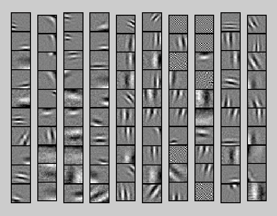
That’s the kind of thing sparse filtering learns from image patches

The downside of multi-layer neural networks is that they’re quite complicated. Specifically, the setup is not the easiest thing, there’re among slower methods as far as we know, and there are many parameters to tune.

Sparse filtering attempts to overcome these difficulties. The difference is, it does not explicitly attempt to construct a model of the data distribution. Instead, it optimizes a simple cost function - the sparsity of L2-normalized features. It’s simple, rather fast and it seems to work.

The hyperparams to choose are:

A number of layers A number of units in each layer

Then you run the optimizer, and it finds the weights. You do a feed-forward step using those weights and you get a new layer, possibly an output layer. Then you feed the output to the classifier and that’s it.

Black Box Competition

The train set for this competition is notably small (1000 examples), as the challenge is structured for unsupervised learning: there’s 140k unlabelled examples. The point is to use them so that they help achieve better classification score.

We trained a two layer sparse filtering structure. Layer one and two both have 100 dimensions. We tried other combinations, for example 400/80 (slightly better) and three layers: 100/100/100 (much worse).

Then we trained a random forest on resulting features. Our code is available at Github.

100/100 using extra data with 300 trees in the forest will get you a score around 0.52, enough to beat the best benchmark. Without extra data you’ll get 0.48, which is still pretty good and much faster.

Some technicalities

• When downloading Sparse Filtering from Github, make sure to get common dir. It’s a separate repository.

• Authors suggest preprocessing data by removing a DC component from each example, that is, its mean value. It makes sense for multimedia data like images, but not necessarily for general data. We found it’s better to skip this step here.

• Most of the time running will be spent in minimizing objective function using minFunc (it’s in common/ dir). You can edit sparseFiltering.m to reduce the number of iterations to make it run faster and the number of so called corrections if you run out of memory:

By default, minFunc uses a large number of corrections in the L-BFGS method. For problems with a very large number of variables, the ‘Corr’ parameter should be decreased (i.e. if you run out of memory on the 10th iteration, try setting ‘Corr’ to 9 or lower).

optW = minFunc(@SparseFilteringObj, optW(:), ...
 struct('MaxIter', 100, 'Corr', 10), X, N);

• You’ll probably get a RCOND warning from minFunc. It means that there is a problem with the data, but everything works anyway.

   Warning: Matrix is close to singular or badly scaled.
   Results may be inaccurate. RCOND = 4.125313e-018.

• If you’d like to use extra data, you might want to convert it to .mat format for reading in Matlab. It can be done with scipy.io.savemat function.

*It’s worth noting that computers became better at recognizing hand-written digits than humans (we’re talking about MNIST dataset here).